Background
The given dataset comes from the Office of Airline Information, Bureau of Transportation Statistics (BTS). It consists of contains on-time arrival data for non-stop domestic flights by major air carriers, monthly from 1987 to 2017, and provides information such as departure and arrival delays, origin and destination airports, flight numbers, scheduled and actual departure and arrival times, canceled or diverted flights, taxi-out and taxi-in times, air time, and non-stop distance. The data is very sizable, since it spans around 30 years and each year contains millions of flights. After June 2003, BTS starts to log more data for each flight, including “cause of delay”. I want to look at all delayed flights and try to predict the cause of delay.
To do this, I used random forests, as it is usually quick to train, performs implicit feature selection, works well with different types of variables, and addresses some of the shortcomings of classification and regression trees. By aggregating many perturbed trees to prevent overfitting and correlation between trees, it can reduce the variance as well. I will tune the parameters to try and get the best possible classifier.
Data cleaning and exploration
I got rid of all cancelled and diverted flights. I then dropped all flights that did not arrive late, because those observations corresponded with NA values for the cause of delay variables. After this, the dimension of my data was 97,699 by 36. Now, a big issue I faced was that for any given flight that arrived late, there were multiple reasons why it ran late. For example, one flight could have ran 10 minutes late due to a security delay, an additional 30 minutes late due to weather delay, and another 5 minutes away due to a carrier delay. So I currently had no way to try and predict a sole reason why a flight was late because there was not a sole reason. What I did to try and fix this was look at the largest cause of delay for a flight and make a variable that reflected that known as max_delay. To continue with the previous example, max_delay would have value “weather delay” because that was the largest cause of delay for the trip.
To feel comfortable doing this, I had to make sure that for most flights, the largest cause of delay was much greater than the second largest cause of delay i.e. that few flights would have “weather delay” equal 30 minutes while “security delay” was 25 minutes. If, in general, there is a clear cause of delay, I would be ok with creating my max_delay variable. Thus, I took the difference of the largest cause of delay with the second largest cause of delay for each flight. I then plotted the differences, which you can see below. With this plot, I felt comfortable proceeding in my data cleaning (there is also an issue with compounding of causes for delay. For example, a 5 minutes security delay could lead to a 15 minute carrier delay, etc. so a ‘main’ cause of delay could be a byproduct of a small delay. I chose to only note this problem for simplification).
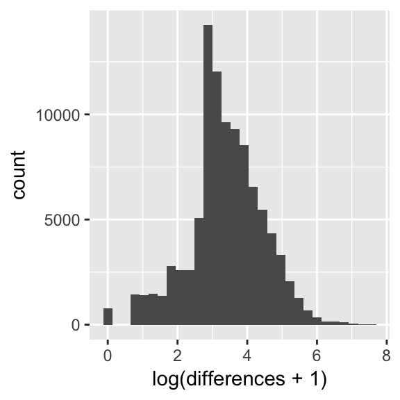
Figure 1: Differences between largest and second largest cause of delay for each flight
Below is the summary of the differences between largest and second largest cause of delay
##    Min. 1st Qu.  Median    Mean 3rd Qu.    Max.
##    0.00   16.00   27.00   49.72   57.00 1933.00
Now, I also had a two variables that represented the origin state and the destination state. Due to the number of levels, it would be infeasible to include as is in the model. I could either make about 100 indicator variables for each level of the two variables, or I could bin the states into four regions (midwest, west, northeast, south) and then make 8 indicator variables. I tried both to see if there would be a big difference in the results.
The final variables I included: Indicators for region (or state), Airline, Indicator for a late departure or not (binary), Lateness of arrival in minutes, Time spent in air in minutes, Time of departure in minutes past midnight, Time of arrival in minutes past midnight, Reason for delay (factor with 5 levels).
I had hopes that including time of arrival would help the classifier detect a trend in time zones if one existed i.e so that it doesn’t say “any late flight that travels more than 3 hours will be late due to x”, because there might be a difference if the destination is hours behind the origin or hours ahead of the origin.
One small thing to notice is the issue of class imbalance. Aircraft and NAS delays combine for less than 4% of the training data, with similar proportions in the testing data. RF might think to ignore those classes and always predict the majority class because it will tend to be correct. A couple of issues to solve this would be undersampling (sampling such that the majority classes have a similar number of observations as the minority class), which would leave too little data, or oversampling (continually sampling the minority class with replacement so that it has a sizable number of observations), which would give me more observations than I wanted to my tiny little computer. I could also try to add class weights, which penalizes the classifier more for misclassifying a minority class, thus making it focus more on that class.
# Imbalanced classes in training data
region_train %>% select(max_delay) %>% count(max_delay) %>% mutate(perc = n / sum(n) * 100)
## # A tibble: 5 x 3
## max_delay n perc
## <fct> <int> <dbl>
## 1 aircraft 108 0.158
## 2 carrier 26366 38.6
## 3 nas 2273 3.32
## 4 security 21704 31.7
## 5 weather 17938 26.2Model
Below includes a table with training and testing error for each parameter combination. Training data was 70% of the original data with 68,398 rows while the testing had 29,310 rows. Recall that I had two datasets, one which included an indicator for each origin and departure state (111 predictors total), which the other had an indicator for each origin and departure region (15 predictors total). When implementing RF without tuning, the MSE for the region data was around .33 while the state data was about .32. Because training with state indicators takes a much longer time, I chose to forgo tuning on that data due to the time constraint. Thus, any remaining analysis is done with the region data.
Regarding the tuning on my training data, I used the tune_RF function that searches for the best mtry, which is the number of variables randomly sample as candidates at each split. You usually do not want this too high. I tuned the value of mtry for three different values of ntree (the number of trees to grow): 100, 500, and 1000. Below is a plot of the results.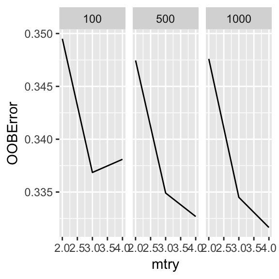
Figure 2: Error based on mtry values faceted by ntree
Below is the confusion matrix and the MSE
##
## optim_mod  aircraft carrier  nas security weather
##   aircraft        0       0    0        0       0
##   carrier        22    9390  423     1456    3905
##   nas             0       6   54       15      29
##   security        8     610  126     7068     775
##   weather        12    1416  391      623    2981
## [1] 0.3349369This does not bode well, as I am sure that the time spent tuning only improved the model an insignificant amount. This is verified after taking the difference between the MSE of the RF with the “optimal” parameters and the base RF; the difference was 0.0009.
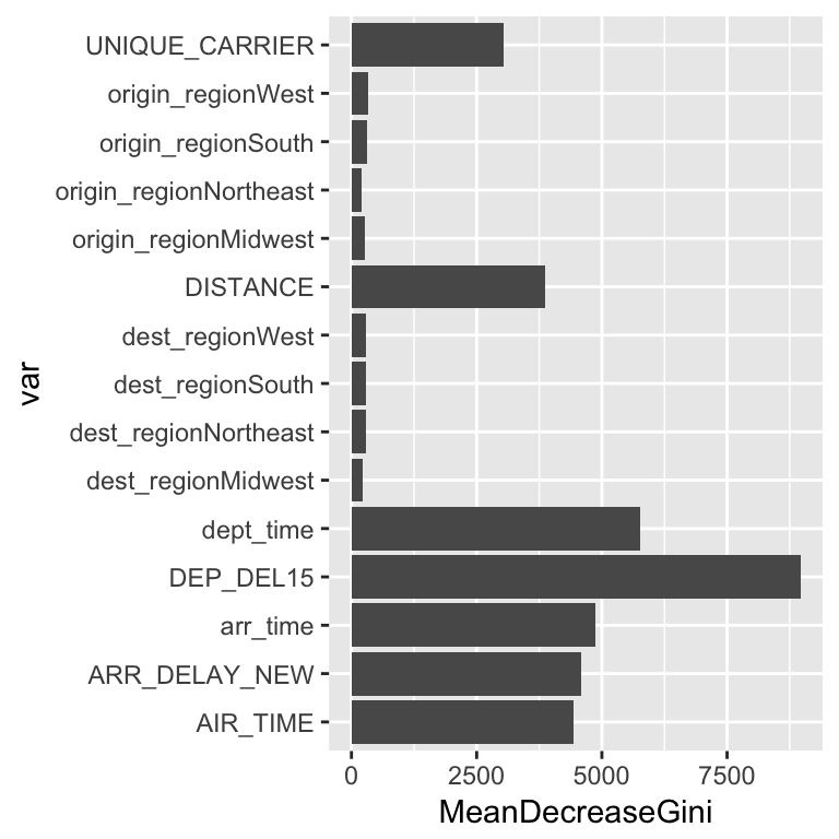
Figure 3: Variable importance
We can see that variables related to departure are important - whether you departed late or not and the time that you departed. I’m surprised that the late departure variable was much more important that the amount of time that you arrived late. The origin or destination is not considered too important, another reason I’m glad I did not keep the 100+ model matrix of indicator variables for each origin and destination state. When looking at the confusion matrix, I can see that the random forests didn’t do too well, as many of the minority classes are frequently misclassified. It never classified an observation as a aircraft delay. As stated before, there are a few methods I could try and would be willing to try in the future, especially class weights.