I forced myself to get rid of Windows after starting grad school. I read plenty of blogs and whatnot explaining why not relying on your mouse (point, click, drag) could make you much more productive while working as a data scientist. I thought only Software Engineers (SWEs) did stuff like that and coding in whatever the heck emacs or vim is. Regardless, I decided to give it a try. Switched to Ubuntu. I’m by no means a terminal whiz, but I know some stuff here and there. Today, I was downloading some data and realized I did most of it without my mouse, which was nice. I also realized I should take the time to make some bash scripts to help do some of the messier things that have annoying syntax.
I wanted to look at data from the Divvy bikeshare program in Chicago. I downloaded all of the 2016 data and put it into a divvy directory I made. This is so I can wrangle the data and help put into practice some of the stuff I read in Python for Data Analysis. The files looked something like this:
- Divvy_Stations_2016_Q1Q2.csv
- Divvy_Stations_2016_Q3.csv
- Divvy_Stations_2016_Q4.csv
- Divvy_Trips_2016_04.csv
- Divvy_Trips_2016_05.csv
- Divvy_Trips_2016_06.csv
- Divvy_Trips_2016_Q1.csv
- Divvy_Trips_2016_Q3.csv
- Divvy_Trips_2016_Q4.csv
as well as some README files. There were all in different folders. I wanted to do something like the following in python
for filename in os.listdir("some_directory"):
    if filename is for trips data:
        with open("some_directory/" + filename, 'r') as f:
        header = next(f)  # Skip the header row.
        cur.copy_from(f, 'rides', sep=',') # read all the data into a table in my database
But some of the trip files ended in months while others ended in quarter numbers. They were also in different folders. I usually would try to click and rename the files, click and make a folder, drag files into the folder, etc. But now I can do the following
$ mkdir data_2016
$ cd data_2016 # note, I should make this mkdir and cd into a nice alias to combine into one step
$ mv ../some_folder/*.csv . # move all csv files in some_folder to the current one
$ repeat last command a couple times
$ wc *Stations* # see the line and word count for all files with Stations in them to notice that new stations were added in Q3 but none in Q4
$ mv Divvy_Stations_2016_Q3.csv Divvy_Stations_2016_Q3Q4.csv # rename file
$ rm Divvy_Stations_2016_Q3.csv # delete file
$ cat <(cat Divvy_Trips_2016_04.csv) <(tail +2 Divvy_Trips_2016_05.csv) <(tail +2 Divvy_Trips_2016_06.csv) > Divvy_Trips_2016_Q2.csv # merge trips from april-june into one csv, only keeping the header from the first file. So now I have trips for each quarter
$ less Divvy_Trips_2016_Q2.csv # check around to make sure it works
$ a little this and a little that
And now I have my data in a nice format and in the same directory! And now I can use the python code above to read all the trips data into my database table. I can then repeat for a stations table. Yay. This isn’t a sort of ‘look at the cool thing I did’ post. It’s just that I decided to learn how to use the terminal about a year ago and it’s nice that I did (and that it’s truly useful). I hope someone who has always had the terminal on their ‘to learn’ list sees this and bumps it up the queue. It can be kinda challenging in the beginning but you can pick it up rather quickly! I’ll have another post soon doing the actual analysis of the data.. nothing big, trying to enjoy the break. Sneak peek: I learned that doing some of the processing via sql is much faster than in pandas. I tried
sql = """SELECT date_trunc('hour', starttime), COUNT(trip_id)
         FROM rides
         GROUP BY date_trunc('day', starttime), date_trunc('hour', starttime)"""
grouped = pd.read_sql(sql, conn)
grouped.index = grouped.date_trunc
grouped.pivot_table(index=grouped.index.hour, columns=grouped.index.date).plot(legend=False, alpha=0.05);
which took about 1.52 seconds while
sql= """SELECT * FROM rides"""
df = pd.read_sql(sql, conn)
df.index = df.starttime
df.groupby([df.index.date, df.index.hour])['trip_id'].count().unstack(level=0).plot(legend=False, alpha=0.05);
took about 35 seconds, 24.9 for reading the data, 9.9 for doing the groupby and rendering the plot. I knew the second attempt would take longer bc I’m reading over 3 million rows vs 8,756 rows in the first attempt but wow that groupby with the large dataset along with the count and unstacking took a long time vs grouping in sql then just using a pivot table. I should brush up on my sql to do more cool stuff before plotting. Oh, and here is the plot (which you will see in the next post).
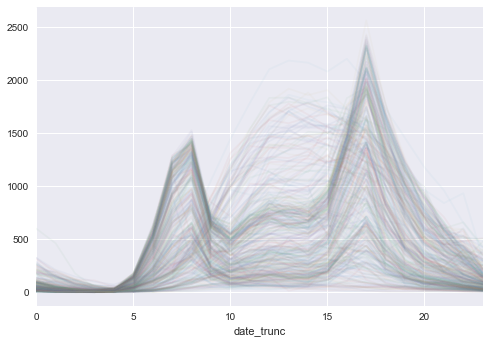
Each line represents a day in the year; x axis represents the hours in a day while the y axis are the number of bikes checked out in that hour. We can see it spikes up at 8 am and 5 pm, which shows school or work commutes. But there are also a number of lines where bike checkouts increase steadily, peaking at noon or 1 pm, then decreasing steadily. These probably are during weekends or days where divvy bikes are used for leisure e.g. tourist or high-schoolers during summer vacation. More to come next time!